
Poisson Regression can be a really useful tool if you know how and when to use it. In this article we’re going to take a long look at Poisson Regression, what it is, and how R programmers can use it in the real world.
Poisson Regression involves regression models in which the response variable is in the form of counts and not fractional numbers. For example, the count of number of births or number of wins in a football match series. Also the values of the response variables follow a Poisson distribution.
The general mathematical equation for Poisson regression is −
log(y) = a + b1x1 + b2x2 + bnxn...
Following is the description of the parameters used −
- y is the response variable.
- a and b are the numeric coefficients.
- x is the predictor variable.
The function used to create the Poisson regression model is the glm() function.
Syntax
> glm(formula,data,family)What Are Poisson Regression Models?
Poisson Regression models are best used for modeling events where the outcomes are counts. Or, more specifically, count data: discrete data with non-negative integer values that count something, like the number of times an event occurs during a given timeframe or the number of people in line at the grocery store.
Count data can also be expressed as rate data since the number of times an event occurs within a timeframe can be expressed as a raw count (i.e. “In a day, we eat three meals”) or as a rate (“We eat at a rate of 0.125 meals per hour”).
Poisson Regression helps us analyze both count data and rate data by allowing us to determine which explanatory variables (X values) have an effect on a given response variable (Y value, the count, or a rate).
Let’s see it with an example
Load Data
We have the in-built data set warpbreaks which describes the effect of wool type (A or B) and tension (low, medium, or high) on the number of warp breaks per loom. Let’s consider breaks as the response variable which is a count of a number of breaks. The wool “type” and “tension” are taken as predictor variables.
> df <- warpbreaks
> head(df)
  breaks wool tension
1     26    A       L
2     30    A       L
3     54    A       L
4     25    A       L
5     70    A       L
6     52    A       L
Visualizing Data
Let’s look at how the data is structured using the ls.str() command:
> ls.str(df)
breaks :  num [1:54] 26 30 54 25 70 52 51 26 67 18 ...
tension :  Factor w/ 3 levels "L","M","H": 1 1 1 1 1 1 1 1 1 2 ...
wool :  Factor w/ 2 levels "A","B": 1 1 1 1 1 1 1 1 1 1 ...
From the above, we can see both the types and levels present in the data. Read this to learn a bit more about factors in R.
Now we will work with the data dataframe. Remember, with a Poisson Distribution model we’re trying to figure out how some predictor variables affect a response variable. Here, breaks is the response variable and wool and tension are predictor variables.
We can view the dependent variable breaks data continuity by creating a histogram:
> hist(df$breaks)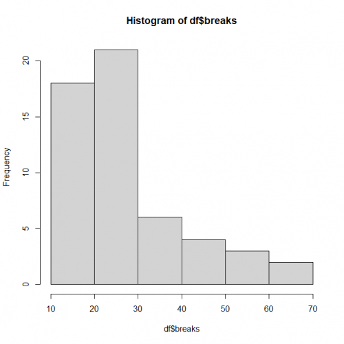
Clearly, the data is not in the form of a bell curve like in a normal distribution.
Let’s check out the mean() and var() of the dependent variable:
# calculate mean
> mean(df$breaks)
Output: [1] 28.14815
# calculate variance
> var(data$breaks)
Output: [1] 174.2041
The variance is much greater than the mean, which suggests that we will have over-dispersion in the model.
Creating Model
Let’s fit the Poisson model using the glm() command.
> model <- glm(df$breaks ~ df$wool + df$tension, family = poisson)
> summary(poisson.model)

Call:
glm(formula = df$breaks ~ df$wool + df$tension, family = poisson)

Deviance Residuals:
    Min       1Q   Median       3Q      Max
-3.6871  -1.6503  -0.4269   1.1902   4.2616

Coefficients:
            Estimate Std. Error z value Pr(>|z|)
(Intercept)  3.69196    0.04541  81.302  < 2e-16 ***
df$woolB    -0.20599    0.05157  -3.994 6.49e-05 ***
df$tensionM -0.32132    0.06027  -5.332 9.73e-08 ***
df$tensionH -0.51849    0.06396  -8.107 5.21e-16 ***
---
Signif. codes:  0 '***' 0.001 '**' 0.01 '*' 0.05 '.' 0.1 ' ' 1

(Dispersion parameter for poisson family taken to be 1)

    Null deviance: 297.37  on 53  degrees of freedom
Residual deviance: 210.39  on 50  degrees of freedom
AIC: 493.06

Number of Fisher Scoring iterations: 4
Conslusion
In the summary, we look for the p-value in the last column to be less than 0.05 to consider the impact of the predictor variable on the response variable. As seen the wool type B having tension-type M and H have an impact on the count of breaks.
This brings the end of this Blog. We really appreciate your time.
Hope you liked it.
Do visit our page www.zigya.com/blog for more informative blogs on Data Science
Keep Reading! Cheers!
Zigya Academy
BEING RELEVANT