In this article, you will learn the basics behind a very popular statistical model, the linear regression.
What is Linear Regression
In statistics, linear regression is a linear approach to modeling the relationship between a scalar response and one or more explanatory variables (also known as dependent and independent variables). The case of one explanatory variable is called simple linear regression; for more than one, the process is called multiple linear regression.
In Linear Regression these two variables are related through an equation, where exponent (power) of both these variables is 1. Mathematically a linear relationship represents a straight line when plotted as a graph. A non-linear relationship where the exponent of any variable is not equal to 1 creates a curve.
The general mathematical equation for a linear regression is −
y = ax + b
Description of the parameters used −
- y is the response variable.
- x is the predictor variable.
- a and b are constants which are called the coefficients.
Example
Moreover this analysis, we will use the cars dataset that comes with R by default. cars is a standard built-in dataset, that makes it convenient to demonstrate linear regression in a simple and easy to understand fashion. You can access this dataset simply by typing in cars in your R console. You will find that it consists of 50 observations(rows) and 2 variables (columns) – dist and speed. Let’s print out the first six observations here.
# head shows only first 6 obervations
> head(cars)
  speed dist
1     4    2
2     4   10
3     7    4
4     7   22
5     8   16
6     9   10
Before we begin building the regression model, it is a good practice to analyze and understand the variables. The graphical analysis and correlation study below will help with this.
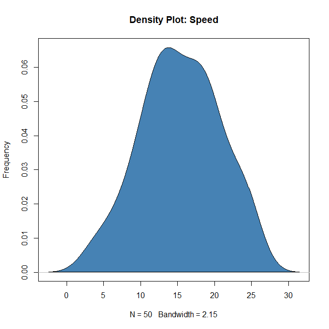
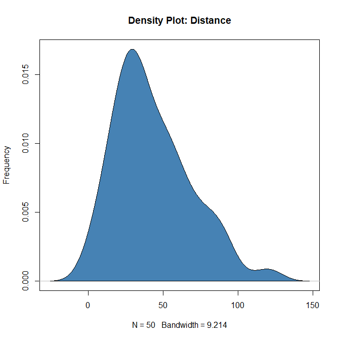
Density plot – Check if the response variable is close to normality
> plot(density(cars$speed), main="Density Plot: Speed", ylab="Frequency")
> polygon(density(cars$speed), col="steelblue")

> plot(density(cars$dist), main="Density Plot: Distance", ylab="Frequency")
> polygon(density(cars$dist), col="steelblue")
Correlation
It is a statistical measure that suggests the level of linear dependence between two variables, that occur in pair – just like what we have here in speed and dist. Correlation can take values between -1 to +1. If we observe for every instance where speed increases, the distance also increases along with it, then there is a high positive correlation between them and therefore the correlation between them will be closer to 1. The opposite is true for an inverse relationship, in which case, the correlation between the variables will be close to -1.
A value closer to 0 suggests a weak relationship between the variables. A low correlation (-0.2 < x < 0.2) probably suggests that much of variation of the response variable (Y) is unexplained by the predictor (X), in which case, we should probably look for better explanatory variables.
cor(cars$speed, cars$dist)  # calculate correlation between speed and distance
#> [1] 0.8068949
Building Linear Model
Now that we have seen the linear relationship pictorially in the scatter plot and by computing the correlation, let’s see the syntax for building the linear model. The function used for building linear models is lm(). The lm() function takes in two main arguments, namely: 1. Formula 2. Data. The data is typically a data.frame and the formula is an object of class formula. But the most common convention is to write out the formula directly in place of the argument as written below.
Description
lm is used to fit linear models. It can be used to carry out regression, single stratum analysis of variance and analysis of covariance (although aov may provide a more convenient interface for these).
Usage
lm(formula, data, subset, weights, na.action,
   method = "qr", model = TRUE, x = FALSE, y = FALSE, qr = TRUE,
   singular.ok = TRUE, contrasts = NULL, offset, ...)
Arguments
| Values | Description |
| formula | an object of class "formula" (or one that can be coerced to that class): a symbolic description of the model to be fitted. |
| data | an optional data frame, list or environment (or object coercible by as.data.frame to a data frame) containing the variables in the model. If not found in data, the variables are taken from environment(formula), typically the environment from which lm is called. |
| subset | an optional vector specifying a subset of observations to be used in the fitting process. |
| weights | an optional vector of weights to be used in the fitting process. Should be NULL or a numeric vector. |
na.action | a function that indicates what should happen when the data contain NAs. The default is set by the na.action setting of and is if that is unset. |
| method | the method to be used; for fitting, currently only method = "qr" is supported; method = "model.frame" returns the model frame (the same as with model = TRUE, see below). |
# build linear regression model on full data
> linearModel <- lm(dist ~ speed, data=cars)
> linearModel
 Call:
 lm(formula = dist ~ speed, data = cars)

 Coefficients:
 (Intercept)        speed
     -17.579        3.932
Now that we have built the linear model, we also have established the relationship between the predictor and response in the form of a mathematical formula for Distance (dist) as a function for speed. For the above output, you can notice the ‘Coefficients’ part having two components: Intercept: -17.579, speed: 3.932 These are also called the beta coefficients. In other words,
dist = Intercept + (β ∗ speed)
=> dist = −17.579 + 3.932∗speed
Linear Regression Diagnostics
Now the linear model is built and we have a formula that we can use to predict the dist value if a corresponding speed is known. Let’s begin by printing the summary statistics for linearModel.
> summary(linearModel)

Call:
lm(formula = dist ~ speed, data = cars)

Residuals:
    Min      1Q  Median      3Q     Max
-29.069  -9.525  -2.272   9.215  43.201

Coefficients:
            Estimate Std. Error t value Pr(>|t|)
(Intercept) -17.5791     6.7584  -2.601   0.0123 *
speed         3.9324     0.4155   9.464 1.49e-12 ***
---
Signif. codes:  0 '***' 0.001 '**' 0.01 '*' 0.05 '.' 0.1 ' ' 1

Residual standard error: 15.38 on 48 degrees of freedom
Multiple R-squared:  0.6511,    Adjusted R-squared:  0.6438
F-statistic: 89.57 on 1 and 48 DF,  p-value: 1.49e-12

> AIC(linearModel)
[1] 419.1569

> BIC(linearModel)
[1] 424.8929
How to know if the model is best fit for your data?
The most common metrics to look at while selecting the model are:
| STATISTIC | CRITERION |
|---|---|
| R-Squared | Higher the better (> 0.70) |
| Adj R-Squared | Higher the better |
| F-Statistic | Higher the better |
| Std. Error | Closer to zero the better |
| t-statistic | Should be greater 1.96 for p-value to be less than 0.05 |
| AIC | Lower the better |
| BIC | Lower the better |
| Mallows cp | Should be close to the number of predictors in model |
| MAPE (Mean absolute percentage error) | Lower the better |
| MSE (Mean squared error) | Lower the better |
| Min_Max Accuracy => mean(min(actual, predicted)/max(actual, predicted)) | Higher the better |
Now we can predict the distance for any speed
predict() Function
Syntax
The basic syntax for predict() in linear regression is −
Usage
predict(object, newdata)
| Values | Description |
object | the object is the formula that is already created using the lm() function. |
newdata | newdata is the vector containing the new value for the predictor variable. |
Let’s predict the amount of distance coverd at a speed of 100 mph
> a <- data.frame(speed = c(10, 100, 1000))
> a
  speed
1    10
2   100
3  1000

> predict(linearModel, a)
         1          2          3
  21.74499  375.66178 3914.82966
As you can see we got the amount of distance which will be covered by the car at a speed of 10mph, 100mph, 1000mph.
Visualize the Regression Graphically
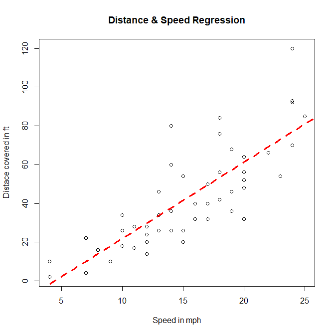
# ploting the distance speed plot with cars dataset
> plot(cars$speed, cars$dist, xlab="Speed in mph", ylab="Distace covered in ft",
  main="Distance & Speed Regression")

# Creating a linear model
> linearModel <- lm(dist~speed, data=cars)
> linearModel

Call:
lm(formula = dist ~ speed, data = cars)

Coefficients:
(Intercept)        speed
    -17.579        3.932

> abline(linearModel, col="red", lty=2, lwd=3)

Conclusion
Hence, we show what is Linear Regression in R, what is Correlation, and how to build your own linear model along with how to diagnose your model whether it is the best fit or not. We also show how to predict values with the model we built and see the result. and in last we represented our linear regression using plot() function.
This brings the end of this Blog. We really appreciate your time.
Hope you liked it.
Do visit our page www.zigya.com/blog for more informative blogs on Data Science
Keep Reading! Cheers!
Zigya Academy
BEING RELEVANT